Kernel Density Estimation with Python from Scratch

Kernel density estimation (KDE) is a statistical technique used to estimate the probability density function of a random variable. It creates a smooth curve from discretely sampled data that reflects the underlying density distribution. KDE is widely used in various fields, including signal processing, statistics, machine learning, data visualization, etc.

Given a set of independent and identically distributed samples $x = \{x_1, x_2, \cdots, x_n\}$, the KDE process can be formulated as:

Where $K$ is the kernel function that satisfies $\int_{-\infty}^{\infty} K(t)dt = 1$. Essentially, for a specific location of $\hat{f}$, the kernel $K$ is assigning a weight for any $x_i$ regarding their distance to $x$. $h$ is a bandwidth parameter, controlling that distance. If this formula is not clear enough, Matthew Conlen's interactive website Kernel Density Estimation provides quite an intuitive insight into the KDE process.

There are several open-source Python libraries available for performing kernel density estimation (KDE), including scipy, scikit-learn, statsmodel, and KDEpy. A blog post by Jake VanderPlas provides a comparison of the algorithms and APIs offered by these libraries. If you want to understand the underlying process of KDE, this post will guide you through writing a KDE process from scratch using Python (although we will still import scipy's optimize function to minimize a function, you can implement your own Golden-Selection search if desired).

First, we need to import some necessary libraries and set the random seed:

import numpy as np
import pandas as pd
import matplotlib.pyplot as plt
from scipy import stats, optimize

rand_seed = 100

Then we are going to generate some datasets for testing. We created four datasets, each containing 100 randomly selected data points drawn from a specific distribution. One distribution is a standard normal distribution, while the other three are bimodal, consisting of normal, exponential, and uniform distributions. The real distribution is returned in the form of probability density functions (PDFs) for visualization.

def make_data_normal(data_count=100):
    np.random.seed(rand_seed)
    x = np.random.normal(0, 1, data_count)
    dist = lambda z: stats.norm(0, 1).pdf(z)
    return x, dist

def make_data_binormal(data_count=100):
    alpha = 0.3
    np.random.seed(rand_seed)
    x = np.concatenate([
        np.random.normal(-1, 2, int(data_count * alpha)),
        np.random.normal(5, 1, int(data_count * (1 - alpha)))
    ])
    dist = lambda z: alpha * stats.norm(-1, 2).pdf(z) + (1 - alpha) * stats.norm(5, 1).pdf(z)
    return x, dist

def make_data_exp(data_count=100):
    alpha = 0.3
    np.random.seed(rand_seed)
    x = np.concatenate([
        np.random.exponential(1, int(data_count * alpha)),
        np.random.exponential(1, int(data_count * (1 - alpha))) + 1
    ])
    dist = lambda z: alpha * stats.expon(0).pdf(z) + (1 - alpha) * stats.expon(1).pdf(z)
    return x, dist

def make_data_uniform(data_count=100):
    alpha = 0.3
    np.random.seed(rand_seed)
    x = np.concatenate([
        np.random.uniform(-1, 1, int(data_count * alpha)),
        np.random.uniform(0, 1, int(data_count * (1 - alpha)))
    ])
    dist = lambda z: alpha * stats.uniform(-1, 1).pdf(z) + (1 - alpha) * stats.uniform(0, 1).pdf(z)
    return x, dist

x_norm, dist_norm = make_data_normal()
x_binorm, dist_binorm = make_data_binormal()
x_exp, dist_exp = make_data_exp()
x_uni, dist_exp = make_data_uniform()

Let's see what these distributions look like:

fig, ax = plt.subplots(1, 4, figsize=(12, 3))
names = ['Normal', 'Bi-normal', 'Exponential', 'Bi-Uniform']
for i, d in enumerate([dist_norm, dist_binorm, dist_exp, dist_uni]):
    x = np.linspace(-8, 8, 100)
    ax[i].fill(x, d(x), color='C0', alpha=0.5)
    ax[i].set_ylim(0, 1)
    ax[i].set_xlim(-8, 8)
    ax[i].set_xlabel('x')
    ax[i].set_ylabel('p(x)')
    ax[i].set_title(names[i])
fig.tight_layout()
fig.show()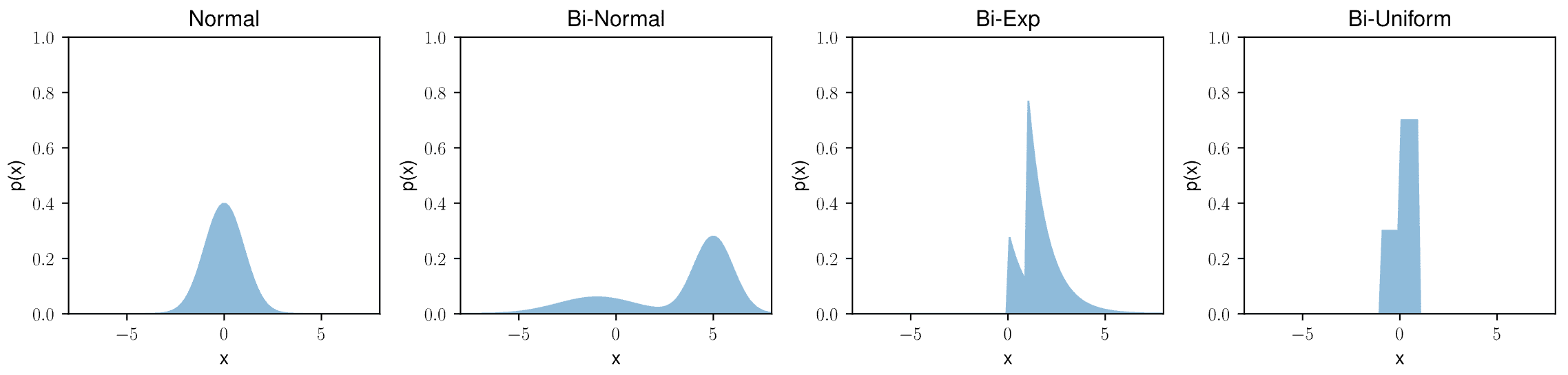

The probability of selecting a value of x at each sample attempt is represented by p(x). We will now define some kernel functions. We will consider four common kernel functions: gaussian, epanechnikov, cosine, and linear. In most cases, you can choose either gaussian or epanechnikov. It's also worth noting that the choice of the kernel function is not as important for the performance of KDE as the bandwidth. The differences in results between different kernels are subtle.

def kernel(k: str):
    """Kernel Functions.
    Ref: https://en.wikipedia.org/wiki/Kernel_(statistics)

    Args:
        k (str): Kernel name. Can be one of ['gaussian', 'epanechnikov', 'cosine', 'linear'.]
    """

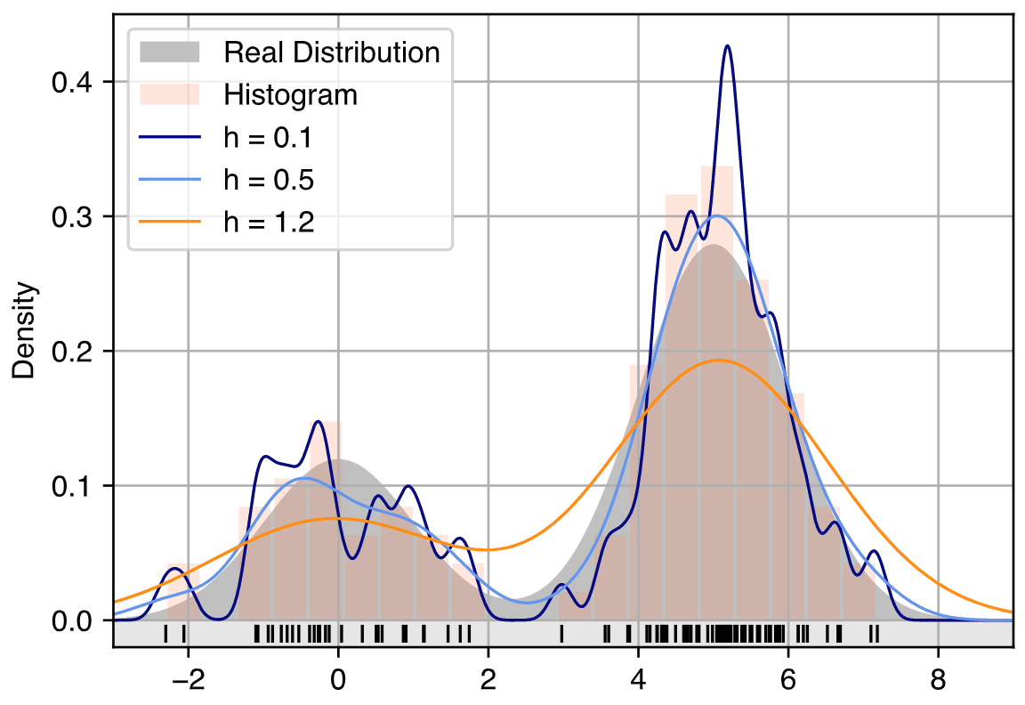
    if k not in ['gaussian', 'epanechnikov', 'cosine', 'linear']:
        raise ValueError('Unknown kernel.')

    def bounded(f):
        def _f(x):
            return f(x) if np.abs(x) <= 1 else 0
        return _f

    if k == 'gaussian':
        return lambda u: 1 / np.sqrt(2 * np.pi) * np.exp(-1 / 2 * u * u)
    elif k == 'epanechnikov':
        return bounded(lambda u: (3 / 4 * (1 - u * u)))
    elif k =='cosine':
        return bounded(lambda u: np.pi / 4 * np.cos(np.pi / 2 * u))
    elif k == 'linear':
        return bounded(lambda u: 1 - np.abs(u))

You can check the size of the kernels from the source. bounded is a wrapper function that intends to crop the function to make it satisfy |x| <= 1. Next, we will look at the bandwidth parameter h of the kernel function. The following picture demonstrates how the KDE results are affected drastically by bandwidth. A larger h will make the curve smoother or even over-smoothing, a smaller h will make the curve sharper, while under-smoothing will lead to unwanted spikes.

The choice of h is quite important to the KDE result. Through trial and error, you can always find a good fit for the dataset. But what if we want an algorithm that automatically gives us an optimal bandwidth for a given dataset? Here we consider three methods: Scott's rule of thumb ¹, Silverman's rule of thumb ², and MLCV (Maximum Likelihood Cross Validation) ³ method.

def bw_scott(data: np.ndarray):
    std_dev = np.std(data, axis=0, ddof=1)
    n = len(data)
    return 3.49 * std_dev * n ** (-0.333)

def bw_silverman(data: np.ndarray):
    def _select_sigma(x):
        normalizer = 1.349
        iqr = (stats.scoreatpercentile(x, 75) - stats.scoreatpercentile(x, 25)) / normalizer
        std_dev = np.std(x, axis=0, ddof=1)
        return np.minimum(std_dev, iqr) if iqr > 0 else std_dev
    sigma = _select_sigma(data)
    n = len(data)
    return 0.9 * sigma * n ** (-0.2)

def bw_mlcv(data: np.ndarray, k):
    """
    Ref: https://rdrr.io/cran/kedd/src/R/MLCV.R
    """
    n = len(data)
    x = np.linspace(np.min(data), np.max(data), n)
    def mlcv(h):
        fj = np.zeros(n)
        for j in range(n):
            for i in range(n):
                if i == j: continue
                fj[j] += k((x[j] - data[i]) / h)
            fj[j] /= (n - 1) * h
        return -np.mean(np.log(fj[fj > 0]))
    h = optimize.minimize(mlcv, 1)
    if np.abs(h.x[0]) > 10:
        return bw_scott(data)
    return h.x[0]

As shown in the code, Scott's rule of thumb is formulated as: $h = 3.49 s n^{(-1/3)}$; Silverman's rule of thumb is formulated as:$h = 0.9 \min(s, IQR / 1.349) n ^{(-1/5)}$. While IQR is the interquartile range, s is the standard derivation of observed data, and n is the number of samples. For MLCV method, the goal is to maximize the likelihood of estimated data calculated from leave-one-out estimator. This post by Niranjan is a good demonstration of the process. There are also many other methods for choosing the optimal bandwidth, like AMISE (Asymptotic Mean Integrated Squared Error), Taylor bootstrap method, DO-validation, etc. You can check This post by Andrey for further reading.

Next, we come to the KDE function itself.

def kde(data, k=None, h=None, x=None):
    """Kernel Density Estimation.

    Args:
        data (np.ndarray): Data.
        k (function): Kernel function.
        h (float): Bandwidth.
        x (np.ndarray, optional): Grid. Defaults to None.

    Returns:
        np.ndarray: Kernel density estimation.
    """
    if x is None:
        x = np.linspace(np.min(data), np.max(data), 1000)
    if h is None:
        h = bw_silverman(data)
    if k is None:
        k = kernel('gaussian')
    n = len(data)
    kde = np.zeros_like(x)
    for j in range(len(x)):
        for i in range(n):
            kde[j] += k((x[j] - data[i]) / h)
        kde[j] /= n * h
    return kde

This kde function should looks easier than you think. With the above preparations, we now have four datasets, four kernel functions, and three bandwidth selection methods. Let's put them all together, record the MSEs and compare their KDE results with matplotlib.

data = [
    ('Normal', make_data_normal),
    ('Bimodal (Normal)', make_data_binormal),
    ('Bimodal (Exp)', make_data_exp),
    ('Bimodal (Uniform)', make_data_uniform)
]
kernels = [
    ('Gaussian', kernel('gaussian')),
    ('Epanechnikov', kernel('epanechnikov')),
    ('Cosine', kernel('cosine')),
    ('Linear', kernel('linear'))
]
bw_algorithms = [
    ('Scott', bw_scott),
    ('Silverman', bw_silverman),
    ('MLCV', bw_mlcv),
]
mses = []

def run_kde(ax, data, kernel):
    x, dist = data[1]()
    x_plot = np.linspace(np.min(x) * 1.05, np.max(x) * 1.05, 1000)
    ax.grid(True)
    ax.fill_between(x_plot, dist(x_plot), fc='silver', alpha=0.5)
    ax.plot(x, np.full_like(x, -0.02), '|k', markeredgewidth=1)
    ax.hist(x, density=True, alpha=0.2, bins=20, rwidth=0.9)
    for bw in bw_algorithms:
        if bw[0] == 'MLCV':
            h = bw[1](x, kernel[1])
        else:
            h = bw[1](x)
        x_kde = kde(x, kernel[1], h=h, x=x_plot)
        mse = np.mean((dist(x_plot) - x_kde) ** 2)
        mses.append({
            'data': data[0],
            'kernel': kernel[0],
            'bw_algorithm': bw[0],
            'h': round(h, 5),
            'mse': round(mse * 1000, 5), # To make differences more noticable
        })
        ax.plot(x_plot, x_kde, linewidth=1, label='$h_{\mathrm{' + bw[0] + '}} = ' + str(round(h, 5)) + '$')
    ax.legend(loc='best', fontsize='small')
    ax.set_title(f'{data[0]}, {kernel[0]}')

fig, axs = plt.subplots(len(data), len(kernels), figsize=(16, 12))

for i, d in enumerate(data):
    for j, k in enumerate(kernels):
        run_kde(axs[i, j], d, k)
    for bw in bw_algorithms:
        avg_h = np.mean([m['h'] for m in mses if m['data'] == d[0] and m['bw_algorithm'] == bw[0]])
        avg_mse = np.mean([m['mse'] for m in mses if m['data'] == d[0] and m['bw_algorithm'] == bw[0]])
        mses.append({
            'data': d[0],
            'kernel': '-',
            'bw_algorithm': bw[0],
            'h': round(avg_h, 5),
            'mse': round(avg_mse, 5),
        })

fig.tight_layout()
fig.show()
fig.savefig('eval.pdf')
pd.DataFrame(mses).to_csv('eval.csv', index=False)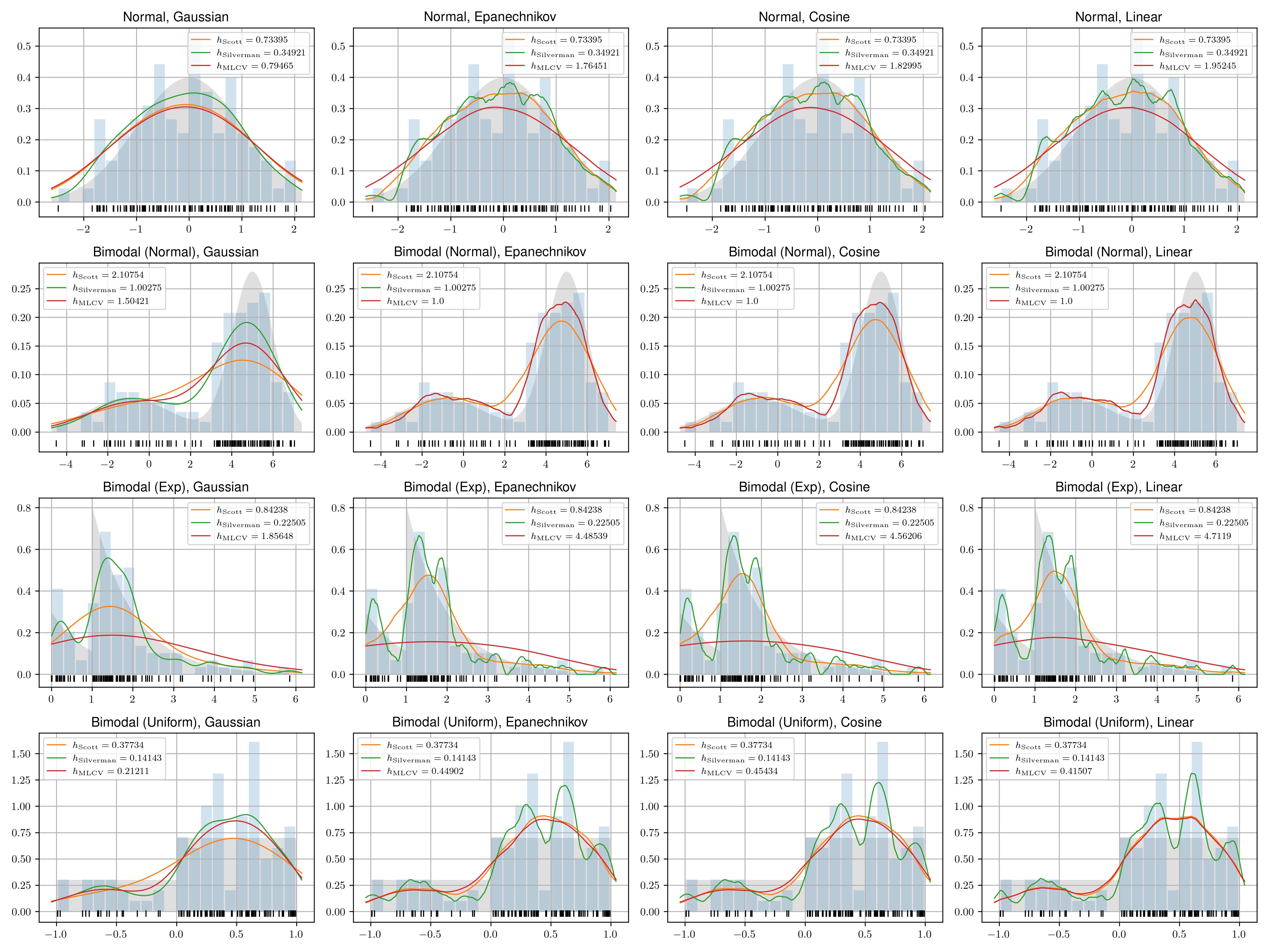

Here we can compare the KDE results of different methods with the real distribution and the histogram. If you followed these steps, you should also be able to see the Mean Square Error (MSE) of each method, kernel and dataset combination in the eval.csv file. The code is also available at https://github.com/billchen2k/KDEBandwidth.

To Sum Up

The results show that Silverman's method is a simple and effective option in most cases. While the maximum likelihood cross-validation (MLCV) method is more mathematically sound, it is much more computationally expensive. Silverman's method is also the default algorithm for selecting the bandwidth in many open-source libraries. The choice of bandwidth selection method has been a topic of intense debate among statisticians during the 1960s and 1970s. If you are interested, you can refer to Scott's textbook on density estimation ⁴. Recent research may have focused more on multivariate density estimation and the combination of cross-validation and plug-in methods.